Bringing Life to Data & Knowledge Graphs With Time Tuples

April 16, 2026

A static graph can tell you what is connected to what. It cannot tell you when those connections formed, when they ended, or what is scheduled to exist in the future. This article explores how promoting timestamp traits from nodes to reified relationships transforms a static snapshot into a temporally-aware model — one that supports point-in-time comparison, historical analysis, future-state planning, and the inference of semantic anti-predicates when nodes die.

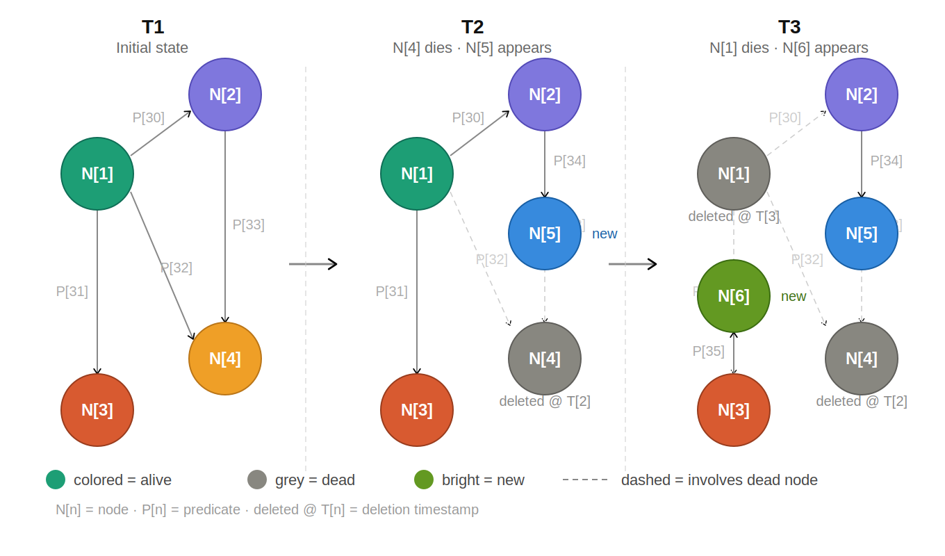
Figure 1: A graph evolving across three points in time (T1 → T2 → T3) — overview

Author: Frank Guerino

From Semantic Expressiveness to Temporal Expressiveness: Building on Prior Work

In the article Data Compilation and Data-Driven Synthesis, I explored how promoting a Node’s Data Type to the reified relationship — rather than leaving it solely as a descriptive node trait — produced richer, more expressive 5-tuples. The result was that the reified relationship carried enough information to generate meaningful semantic sentences on its own, without needing to reach back into the nodes themselves to assemble a complete thought. The promotion was intentional and purpose-driven: the goal was semantic expressiveness, and elevating Data Type to the relationship level was the design decision that achieved it.

That article also introduced NOUNZ, a Data Compiler I designed and built to operationalize this idea at scale — automatically generating 5-tuple reified semantic relationships from structured data sources, producing Knowledge Profiles rich enough to support reasoning, search, and natural language description across large enterprise data graphs.

In Understanding Reified Relationships, N-Tuples, and How They Give Life to Data, I deepened the conceptual foundation — examining what reification means, why it matters, and how the depth of an N-tuple determines the expressiveness and analytical value of a relationship. A key principle established there is that trait promotion is a design decision, not a default. Certain traits belong on nodes. Others, when promoted to the reified relationship, unlock capabilities that simply are not available when those traits remain node-bound.

This article applies that same principle to a different trait and a different goal. Rather than promoting Data Type for semantic expressiveness, I propose promoting Creation Timestamp and Deletion Timestamp for temporal expressiveness. When timestamps live only on nodes, they describe the lifecycle of the node itself. Useful for node-level auditing, but limited in analytical scope. When those same timestamps are promoted to the reified relationship, they describe the lifecycle of the connection — when this specific relationship between these two nodes came into existence and when it ceased to exist.

It is worth noting that promoting timestamps to the reified relationship does not remove them from the node. The node retains its own timestamps for its own descriptive and auditing purposes. Promotion is additive — the same trait now serves two roles at two different levels of the graph, each answering a different class of question.

The graph gains a memory and a future. It begins to move.

From 5-Tuples to 9-Tuples: The Structural Evolution

The NOUNZ compiler generates reified semantic relationships as 5-tuples with the following structure:

Source Node Data Type
Source Node Identifier
Descriptive Predicate
Target Node Data Type
Target Node Identifier

This structure is powerful because it promotes both the Node’s identifier and its Data Type — a classification that tells you what kind of thing the node is, such as Human, Application, Country, or Organization — to the reified relationship. The result is a relationship that can generate a meaningful semantic sentence without needing to reach back into either node to complete its meaning.

Promoting Creation Timestamp and Deletion Timestamp from node traits to reified relationship traits extends this structure from a 5-tuple to a 9-tuple:

Source Node Data Type
Source Node Identifier
Source Node Creation Timestamp
Source Node Deletion Timestamp
Descriptive Predicate
Target Node Data Type
Target Node Identifier
Target Node Creation Timestamp
Target Node Deletion Timestamp

Figure 2: Structural evolution from the original NOUNZ 5-tuple to the temporal 9-tuple

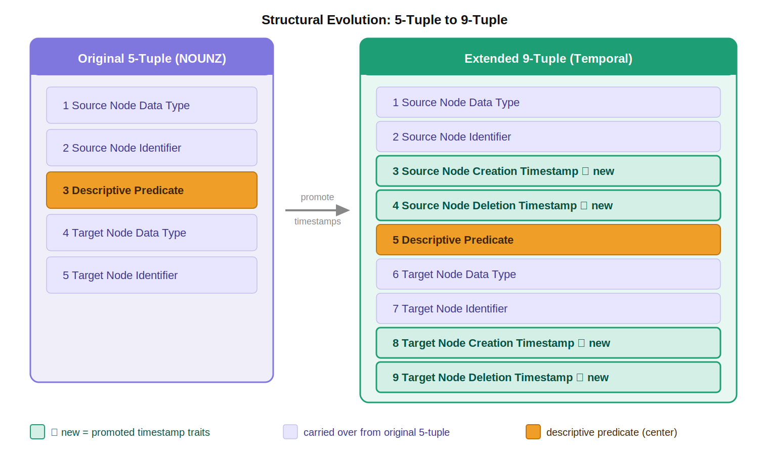
The structure is symmetric: four traits describe the source node, one predicate describes the connection, and four traits describe the target node. The two timestamp traits on each side of the predicate define the lifespan of that node’s participation in the relationship — when it arrived and when, if ever, it departed.

Together, Creation Timestamp and Deletion Timestamp define a precise window of existence for each node within the context of each relationship it participates in. A node whose Deletion Timestamp is null is alive. A node whose Deletion Timestamp is set is dead — it existed, it participated in this relationship, and it is gone. The window between the two timestamps is the node’s life as a participant in that connection.

A note on scope: Nodes can also carry a Modification Timestamp that records when a node’s properties were last changed, providing additional historical context about the node’s evolution over time. I have intentionally omitted Modification Timestamp from the 9-tuple structure presented here in order to keep the concepts as clean and accessible as possible. Creation Timestamp and Deletion Timestamp are sufficient to establish the temporal dimension of the reified relationship — they define when a node’s participation in a relationship began and when it ended. The role of Modification Timestamp in temporal graph modeling is a topic worth exploring in its own right and may be addressed in a future article.

This is what gives the graph its temporal dimension. Every relationship now carries not just what is connected to what, but when each participant arrived, and when each participant left.

What Changes When Timestamps Move to the Relationship

Figure 3a: T1 — the baseline graph with all nodes alive and all relationships active

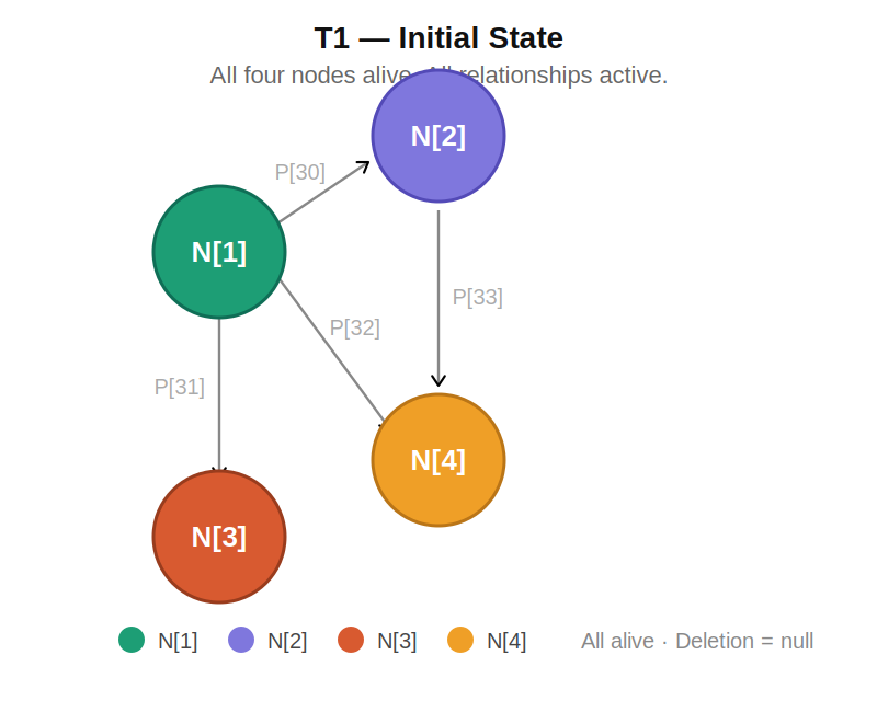
A graph without temporal relationship traits is a photograph. It shows you what exists at the moment the shutter clicked — which nodes are present, which connections are active, what the structure looks like right now. That photograph can be enormously useful. But it cannot show you how the graph got to where it is, what it looked like before, or where it is headed.

When Creation Timestamp and Deletion Timestamp are promoted to the reified relationship, the photograph becomes a film. Each relationship now carries its own temporal identity — an answer to the questions: when did this connection first appear, and when did it end? Across the full graph, those answers compose a timeline. Nodes and relationships appear, evolve, and disappear. Patterns that are invisible in a static snapshot become visible when time is introduced as a dimension of the relationship itself.

This is not a small shift in perspective. It is a fundamental expansion of what the graph can express and what questions it can answer. A static graph supports queries like: what is connected to what, and how? A temporally-aware graph supports a richer class of queries: what was connected to what at a given point in time, what changed between two points in time, and what connections are scheduled to exist in the future?

The Three Temporal States of a Relationship

When timestamps are part of the reified relationship, every relationship in the graph can be understood as existing in one of three temporal states:

Past — the relationship existed at some point but no longer does. Its Creation Timestamp records when it came into being. Its Deletion Timestamp records when it ended. Querying past relationships reveals the history of the graph — what connections once existed, when they were established, and when they ended.

Present — the relationship currently exists. Its Creation Timestamp records when it was established. Its Deletion Timestamp is null — the relationship is alive. The present state of the graph is the familiar static view, now enriched with temporal context about how each connection came to be.

Future — the relationship does not yet exist but is scheduled to. This is perhaps the most powerful and underappreciated of the three states. A data integration that has been designed, approved, and scheduled for implementation at a specific date in the future is a real thing — it has a planned existence, a defined source and target, and a known go-live date. Representing it as a future-dated reified relationship means the graph can answer questions about the planned future state of the enterprise just as readily as it answers questions about the current or historical state.

Figure 3b: The three temporal states of a relationship on a timeline

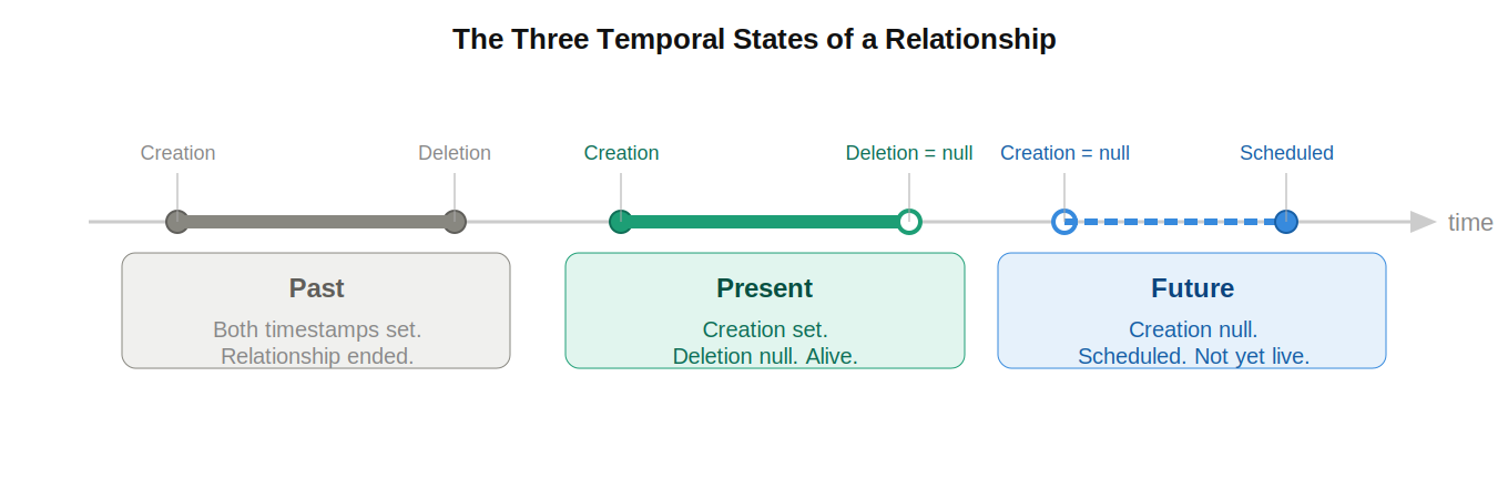
Together, these three states give the graph a complete temporal vocabulary. The same model — the same nodes, the same relationship structure — carries past, present, and future simultaneously.

A Concrete Example: Data Integrations Through Time

Data integrations are among the most natural candidates for temporal relationship modeling. A fully described data integration is itself a reified N-tuple relationship — it has a source node (the system sending data), a target node (the system receiving data), and a rich set of descriptive traits about how the data travels between them: the integration mechanism, the payload, the trigger type, the frequency, the owning team, and more.

Now consider what happens when Creation Timestamp and Deletion Timestamp are added to that reified relationship.

Integration A — established three years ago between a CRM system and a billing platform. Creation Timestamp: three years ago. Deletion Timestamp: null — still active.

Integration B — established two years ago between a legacy reporting system and a data warehouse, but retired six months ago when the legacy system was decommissioned. Creation Timestamp: two years ago. Deletion Timestamp: six months ago.

Integration C — not yet live. A planned integration between a new data lake and an executive reporting tool, scheduled for implementation at a specific date in the future. Creation Timestamp: null. Scheduled Creation Timestamp: a specific date in the future.

A static graph shows Integration A as present, Integration B as absent, and Integration C as absent. A temporally-aware graph tells a richer story: Integration A has been running reliably for three years. Integration B existed, served its purpose, and was retired — its history is preserved. Integration C is a commitment about the future, not yet a reality — but real enough to plan around, model dependencies against, and track toward completion.

Now imagine querying the graph at two separate points in time — say, eighteen months ago and today. The diff between those two snapshots reveals exactly what changed: which integrations were added, which were retired, and which are new commitments. That diff is impact analysis. It is change documentation. It is an audit trail. And it is generated automatically from the temporal structure of the graph itself, without requiring a separate change management system.

Dead Nodes, Deletion Timestamps, and the Inferred Anti-Predicate

Figure 4a: T1 → T2 — N[4] dies, N[5] appears, dashed edges show terminated relationships

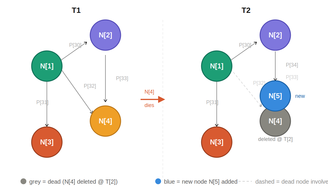
One of the most significant consequences of promoting Deletion Timestamp to the reified relationship is what happens when a node dies — when its Deletion Timestamp is set.

A dead node does not disappear from the graph. It remains present, its Deletion Timestamp marking the moment it ceased to exist as an active participant. This is intentional. Removing dead nodes would destroy historical context — the graph would lose its memory of what once existed and what connected to it. Instead, dead nodes are visually distinguished from living ones. A common convention is to render dead nodes in black or grey, making their status immediately apparent while preserving their presence in the graph for historical analysis and query.

But the implications go further. When a node dies, every active relationship it participated in is affected. And critically, the nature of that effect can be inferred from the relationship type and the cause of the node’s deletion.

Consider Mary and John. Mary is the Spouse of John — an active reified relationship in the graph. Now Mary dies. Her Deletion Timestamp is set.

In a static graph, the Spouse relationship simply ends. But in a temporally-aware graph with semantic relationship types, the death of Mary does not merely terminate the relationship — it transforms it. Because the termination is caused by death rather than separation, the graph can infer:

Mary is no longer John’s Spouse
John is Widowed — not Divorced, not Separated
Mary is John’s Deceased Spouse — a historically accurate description of what she was and what she became

Figure 4b: The anti-predicate — how Mary’s death transforms the Spouse relationship

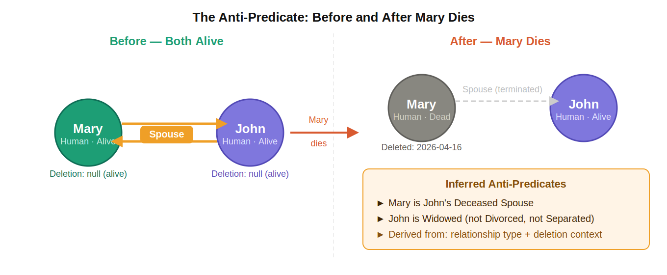
This inferred transformation is what I call the anti-predicate — the semantic inverse or consequence of a relationship’s termination, derived automatically from the relationship type and the deletion context of one of its nodes. The anti-predicate does not need to be explicitly stated because it can be computed. The combination of relationship type plus deletion state carries enough information to generate it.

This is a concrete and implementable pattern in computer science. A trigger on any reified relationship — firing whenever one of its nodes receives a Deletion Timestamp — can evaluate the relationship type and deletion context, then create or annotate the anti-predicate automatically. The specifics of how such triggers are designed, what forms the anti-predicate takes, and how they integrate with graph query engines are rich topics that deserve their own dedicated treatment and will be addressed in a future article.

Figure 4c: T2 → T3 — N[1] dies, N[6] appears, history accumulates across two deletions

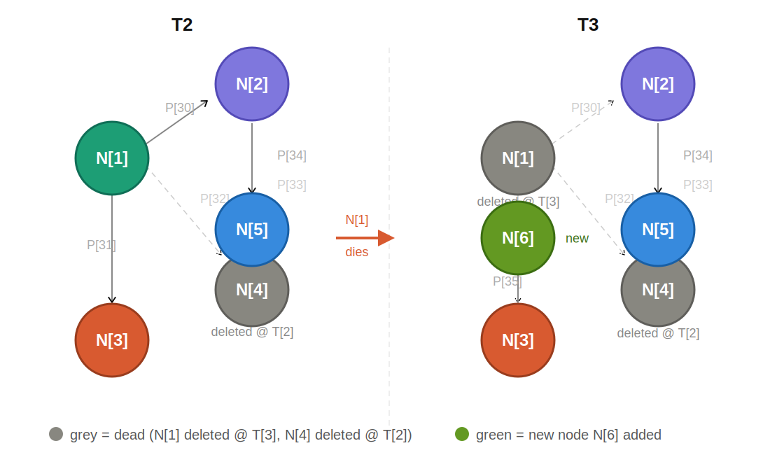
As history accumulates across time points — as shown above moving from T2 to T3 — the graph builds an increasingly rich record. Dead nodes from earlier time points remain present as permanent historical witnesses. New nodes and relationships layer on top of that history. The graph grows not just in breadth but in depth, carrying the full story of how the enterprise has changed.

Point-in-Time Comparison: Understanding Change Between Two Snapshots

One of the most powerful analytical capabilities that temporal relationship traits enable is point-in-time comparison — the ability to query the graph as it existed at two different moments and produce a structured account of what changed between them.

Change impact analysis — before making a planned change to the graph, compare the current state against the proposed future state to understand what relationships will be added, deleted, or modified, and what downstream effects those changes will have.

Audit and compliance — regulatory environments often require organizations to demonstrate that their data landscape was in a specific state at a specific point in time. A temporally-aware graph can answer those questions directly without reconstructing history from logs.

Gap analysis — compare the current state of the graph against a planned or target future state to identify what relationships are missing, what has not yet been implemented, and how far the actual state of the enterprise diverges from its intended architecture.

Trend analysis — compare the graph across multiple points in time to identify patterns: which areas of the enterprise are growing in connectivity, which are becoming simpler, which have not changed at all. Stagnation is as meaningful a signal as growth.

In each of these cases, the analytical value comes directly from the decision to promote timestamps to the reified relationship. Without that promotion, the graph cannot answer when. With it, when becomes a first-class dimension of every query.

The Sense of Motion

There is something worth pausing on that goes beyond the analytical benefits described above. When timestamps are part of the reified relationship, the graph stops being a static artifact and starts behaving like a living model of the enterprise.

Visualized over time, nodes grow and shrink in their connectivity. Relationships appear and fade. Dead nodes — rendered in black or grey, their Deletion Timestamps marking the moment they ceased to participate — remain present as historical witnesses to what once existed. Planned future relationships, their Creation Timestamps still in the future, appear as commitments not yet fulfilled. Clusters form, consolidate, and sometimes dissolve.

Color becomes a natural vocabulary for the temporally-aware graph. Dead nodes — those whose Deletion Timestamp has been set — are rendered in black or grey, immediately distinguishing them from their living counterparts. Living nodes, by contrast, can use color expressively: a node’s color can signal its Data Type, its activity level, its relationship density, or any other trait that aids interpretation. The convention is intuitive — color means life, and the specific color carries meaning about what kind of life. Black or grey means the node’s participation in the graph has ended. This simple visual language transforms a complex graph into something a reader can interpret at a glance, even before examining individual relationships or timestamps.

The graph breathes. This is not merely aesthetic — it is epistemically significant. Motion in the graph reflects motion in the enterprise. When you can see the graph change, you can see the organization change. You can see where investment is flowing, where legacy systems are being retired, where new capabilities are emerging, and where planned work is materializing into reality.

This sense of motion is only possible because the relationships themselves carry temporal identity. A relationship that knows when it was born, when it ended, and when it is scheduled to exist is a relationship that participates in the timeline of the enterprise. Aggregated across thousands of such relationships, the graph becomes something more than an inventory — it becomes a living record of how the enterprise connects, evolves, and grows.

Design Considerations

Introducing temporal traits to reified relationships is a powerful capability, but like all architectural decisions it comes with design considerations worth thinking through before implementation.

Granularity of timestamps — decide upfront what level of precision your timestamps require. For most enterprise graph use cases, date-level precision (YYYY-MM-DD) is sufficient. For high-frequency operational graphs, datetime precision may be needed. Consistency across all relationships in the graph is more important than the specific granularity chosen.

Null handling for future and active relationships — a null Deletion Timestamp means the relationship or node is currently alive. A null Creation Timestamp on a future relationship means it has not yet been established. Define clear conventions for both states and apply them consistently across the graph.

Immutability of Creation Timestamp — once a relationship is created, its Creation Timestamp should be treated as immutable. It is a historical fact, not an editable property. Deletion Timestamp, by contrast, is set at the moment the relationship or node ends.

Retention of dead nodes and relationships — dead nodes and deleted relationships should be retained in the graph rather than removed. Removal destroys historical context and eliminates the point-in-time comparison capabilities described above. Retention with visual distinction — rendering dead nodes in black or grey — preserves the full historical record while keeping the current state of the graph legible.

Anti-predicate handling — decide whether anti-predicates are generated automatically via triggers, computed at query time, or both. Consistency in how anti-predicates are represented across different relationship types is essential for reliable semantic inference.

Tooling alignment — not all graph databases and data compilers handle temporal traits natively. Verify that your tooling supports the temporal query patterns you intend to use before committing to a temporal graph design.

Conclusion

The decision to promote Creation Timestamp and Deletion Timestamp from node traits to reified relationship traits is a small architectural change with large analytical consequences. It does not disrupt the existing model — nodes retain their own timestamps for their own purposes. It adds a new dimension to every relationship in the graph: a temporal identity that answers when this connection came to be and when it ended.

The structural evolution from the original NOUNZ 5-tuple to the 9-tuple introduced here is a natural progression. Data Type was promoted for semantic expressiveness. Timestamps are promoted for temporal expressiveness. Each promotion adds depth to the reified relationship without removing anything from the nodes themselves — promotion is always additive.

With the temporal dimension in place, the graph can represent the past, the present, and the planned future simultaneously. It can be queried at any point in time. It can be compared across two points in time to reveal what changed and how. Dead nodes remain as historical witnesses. Future relationships appear as commitments. And when a node dies, the graph does not merely record its absence — it infers the semantic consequences of that absence through the anti-predicate, generating new meaning from the fact of deletion.

The principle at work here is the same one established in prior articles in this series: trait promotion is a design decision, not a default, and the right decision depends on what you want the graph to be able to express. Promote Data Type, and the graph becomes semantically expressive. Promote timestamps, and the graph becomes temporally expressive.

Give the graph time, and it begins to move.

Published by Guerino Enterprises, LLC – Copyright Guerino Enterprises & Frank Guerino